Solver

DDPM

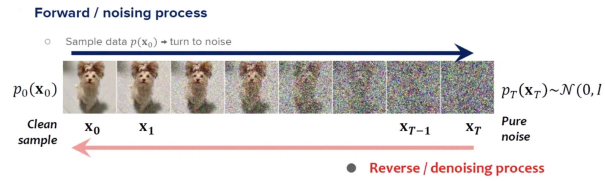
• Forward Process (Noise Addition): This is where the model gradually adds noise to the data, step by step, until the original data is completely turned into noise. This process is typically modeled using a Markov chain.

• Reverse Process (Denoising): In the reverse process, the model learns how to recover the original data from the noisy version, step by step. This is where the generative magic happens—by reversing the noise addition process, the model gradually recovers the original signal, ultimately producing clean data from random noise.

Diffusion models belong to the broader family of probabilistic models, where the generation of data is formulated as a sequence of probabilistic transitions from a simple distribution (like pure noise) to a complex data distribution (such as real images).

How Do Diffusion Models Work?

To better understand diffusion models, let’s break down the steps involved in both the forward and reverse processes.

Forward Process (Adding Noise)

In the forward process, we start with a data point (e.g., an image) and progressively add small Gaussian noise over several time steps. As the process continues, the image becomes increasingly noisy until, at the end of the process, it resembles pure Gaussian noise. For an image \(x_0\), at each time step t, noise is added according to the formula \(x_{t+1}=\sqrt{1-\beta_t}x_t+\beta_t\epsilon\). \(\beta_t\) is called noise schedule, which controls how much noise is added at each step, typically starting with a small amount and increasing as time progresses. \(\epsilon\) is random Gaussian noise. For mathematical convenience, we may write \(\alpha_t=1-\beta_t\), and \(x_{t+1}=\sqrt{\alpha_t}x_t+\sqrt{1-\alpha_t}\epsilon\)

We can rewrite forward process in terms of probability. In this case, \(q(x_{t+1}\vert x_t)=N(x_{t+1}; \sqrt{\alpha_t}x_t,(1-\alpha_t)I)\).

Reverse Process (Denoising)

Once the forward process is defined, the goal of the diffusion model is to learn the reverse process. The reverse process involves learning how to remove the noise step by step, recovering the original data distribution from the noisy version.

Thus, the question becomes acquiring backward probability – \(q(x_t \vert x_{t+1})\). However, if we directly apply bayesian laws, we get \(q(x_t \vert x_{t+1})=\frac{q(x_{t+1} \vert x_{t})q(x_t)}{q(x_{t+1})}\). We don’t know anything about \(q(x_{t+1})\) or \(q(x_t)\).

What we can do is using \(x_0\) as additional information in these probabilities. Instead of solving \(q(x_t \vert x_{t+1})\), we solve \(q(x_t \vert x_{t+1},x_0)\). After bayesian laws we get \(q(x_t \vert x_{t+1},x_0) = \frac{q(x_{t+1} \vert x_{t},x_0)q(x_t \vert x_0)}{q(x_{t+1} \vert x_0)}\). \(q(x_{t+1} \vert x_{t},x_0)\) is the same as \(q(x_{t+1} \vert x_{t})\) due to markov chain property.

It turns out that \(q(x_{t+1} \vert x_0)\) and \(q(x_t \vert x_0)\) can be solved using reparameterization trick. The mathematical derivation of the trick is below.

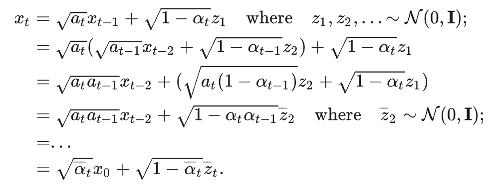
Essentially, we can write \(q(x_{t+1} \vert x_0)\) and \(q(x_t \vert x_0)\) as \(N(x_{t+1};\sqrt{\bar{\alpha}_{t+1}}x_0, (1-\bar{\alpha}_{t+1})I)\) and \(N(x_t;\sqrt{\bar{\alpha}_t}x_0, (1-\bar{\alpha}_t)I)\). After some heavy calculations, we can get \(q(x_t \vert x_{t+1},x_0)=N(x_t;\tilde{\mu}_{t+1}(x_{t+1}),\Sigma_q(t+1)I)\). We can rewrite it as \(q(x_{t-1}\vert x_t,x_0)=N(x_{t-1};\tilde{\mu_t}(x_t),\Sigma_q(t)I)\) where \(\tilde{\mu_t}(x_t)=\frac{1}{\alpha_t}(x_t-\frac{\beta_t}{\sqrt{1-\bar{\alpha}_t}}\bar{z}_t)\). \(\Sigma_q(t)=\frac{(1-\alpha_t)(1-\bar{\alpha}_{t-1})}{1-\bar{\alpha}_t}\).

Training the Diffusion Model

In order to train a model, we must define its loss function. By maximizing the likelihood of data distribution \(log p_{\theta}\) and a series of math deduction, we can get the loss function. The full derivation of loss terms is referenced here

First term is called reconstruction term, which measures how well the reconstructed image match the original image.

Second term is called prior matching term, which describes how well the final latent space \(p_T\) matches standard Gaussian distribution. Normally we treat it as 0 under the assumption that the final output will be random noise after adding multiple small amount of noises.

The third term is called denoising matching term, which matches denoising distribution \(q(x_{t-1}\vert x_t,x_0)\) with model’s prediction \(p_{\theta}(x_{t-1} \vert x_t)\). We can parameterize the mean of model’s prediction as \(p_{\theta}(x_{t-1} \vert x_t)=N(x_{t-1};\tilde{\mu_{\theta}}(x_t,t),\Sigma_q(t)I)\).

Recall that \(q(x_{t-1} \vert x_t,x_0)=N(x_{t-1};\tilde{\mu_t}(x_t),\Sigma_q(t)I)\). Applying KL divergence, we can get the loss function \(\frac{1}{2{\Sigma_q(t)}^2}[{ \parallel \mu_{\theta}-\mu_t \parallel}^2]\).

The author of the paper finds out that we can directly predict noise instead of the mean, which makes the loss function look like this one: \(C[{ \parallel \epsilon_{\theta} - \epsilon_t \parallel }^2]\) where C is a constant.

Sampling from the Diffusion Model

Once trained, the model can generate new data by starting with a random noise sample and iteratively denoising it through the reverse process until a realistic sample is produced. As the model predicts the noise at time t, it will subtract that noise from sampled image to get less noiser image.

Applications of Diffusion Models

Diffusion models have been successfully applied across a wide range of domains. Here are a few notable applications:

1. Image Generation The most prominent use case for diffusion models has been in image generation. Models like DALL·E 2 and Stable Diffusion leverage diffusion techniques to create high-quality, photorealistic images from text descriptions. These models are trained on large datasets of images and learn to generate realistic images by reversing the diffusion process.

2. Super-Resolution and Image Inpainting Diffusion models have also been applied to tasks like image super-resolution (increasing the resolution of low-quality images) and inpainting (filling in missing parts of an image). By learning the reverse diffusion process on images with added noise, these models can recover fine details and generate high-resolution content from low-quality inputs.

3. Audio and Speech Synthesis Diffusion models are also being used to generate audio and speech. By treating sound waves as data and adding noise over time, diffusion models can generate natural-sounding speech or music by reversing the noise process, step by step.

4. Video Generation Generating video frames is a more complex task, but diffusion models are also making strides in this area. Video generation with diffusion models typically involves generating high-quality sequences of frames that are consistent and coherent over time.

Why Are Diffusion Models So Effective?

There are several reasons why diffusion models have become so popular in generative AI:

1. Stability: Unlike GANs, which can suffer from training instability, diffusion models tend to be more stable during training, as they optimize a simpler objective—predicting noise at each step rather than 2 objectives of generating and discriminating images.
2. High-Quality and Diverse Output: Due to its direct operations over continuous distributions and the randomness in the diffusion process, it can generate high-quality and diverse images.

Challenges and Future Directions

While diffusion models have demonstrated significant promise, they are not without challenges:

• Computational Expense: Diffusion models typically require a large number of time steps to generate data, which makes the sampling process computationally expensive. However, researchers are actively working on techniques to reduce this computational cost while maintaining output quality.

• Sampling Speed: Due to the iterative nature of the reverse diffusion process, generating data with diffusion models can be slower than other generative models like GANs. There is ongoing research into speeding up the sampling process.

• Data Efficiency: Diffusion models tend to require a large amount of training data to perform well, which can be a limitation in some cases.

Despite these challenges, diffusion models are rapidly advancing and are likely to remain at the forefront of generative AI research for the foreseeable future.

Conclusion

Diffusion models represent a fascinating and powerful approach to generative AI, offering high-quality and stable generation of diverse data types. Their ability to model complex distributions through a gradual process of noise addition and removal has revolutionized fields like image synthesis, super-resolution, and audio generation. While there are still challenges to overcome, diffusion models are undoubtedly a key part of the future of generative AI, and we can expect to see even more exciting applications in the coming years.

As the field continues to evolve, diffusion models will likely play a crucial role in shaping the next generation of AI-powered creativity and innovation.