AE

Before talking about VAE, first talk about AE model. AE model aims to decompress and compress images via an encoder and a decoder. Its main purpose is for compressing an image, and this structure is effective While this does allow compression and decompression, it misses the potential usage of such model of generating image. Simple idea of generating image is first draw a sample from latent space following a Gaussian distribution, and then use decoder to generate new images based on it. However, the question lies on the image distribution is most likely to differ from Gaussian distribution.

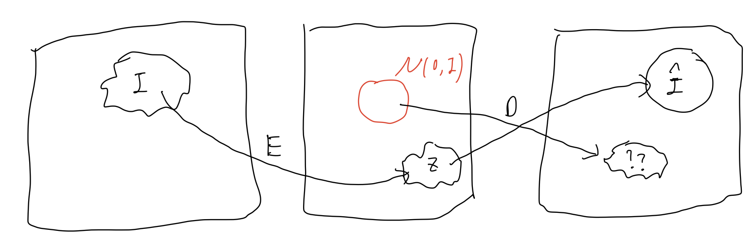
When the model draws a random sample from Gaussian distribution, it’s most likely to map onto a random noise because the encoder doesn’t learn to map image distribution on to Gaussian distribution. The advent of VAE aims to solve this problem.

VAE

Quick explanation

In order to constrain the distribution of images to Gaussian distribution, VAE uses two vectors to represent final Gaussian distributions in latent varaible, \(\mu\) and \(\sigma\), to simplify the constrain. In addition to architectural changes, it adds additional KL loss onto image reconstruction loss in AE to regulate latent distribution to Gaussian distribution, which is \(L={1}/{2}(-1+{\sigma}^2+{\mu}^2-{log {\sigma}}^2)\). Detailed explanation of its loss term, and the application of ELBO will be discussed in the future post.

Experiment

I implemented a simple version of VAE, using only MLP as the encoder and decoder and training on MNIST dataset.

First observation is that the number of dimension in mean and deviation vectors has a significant impact on the quality of image generation.

As the latent space dimention increases, the quality of produced image significantly improves.

However, when we use images with more details to train the model, such as CIFAR10, the model can’t reconstruct the original images. The reconstructed images are instead very blurry.

As I change the size of train dataset, there’s an interesting phenomenon regarding image generation.

We can see that the generated image is like taking the average of the images in a batch. This is probably because when doing back propagation, the model is doing propagation on all images and takes the average of the gradient. Thus, the final image will resemble all the images in the batch.

Causes

As I checked from website, I got to know a phenomenon called posterior collpase. Posterior collapse is when signal from input x to posterior parameters is either too weak or too noisy, and as a result, decoder starts ignoring z samples drawn from the distribution by encoder.

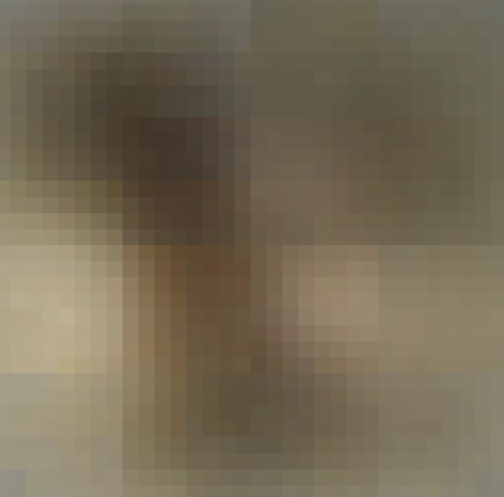
A more evident phenomenon is when the decoder generates an image regardless of the input. Thus, I tested some images on VAE to see whether they produce the same image despite different inputs.

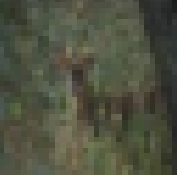
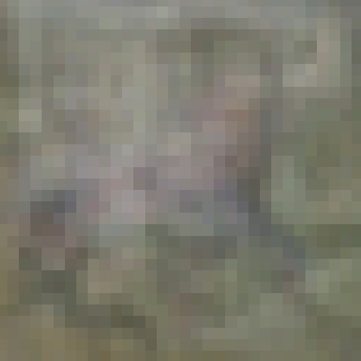
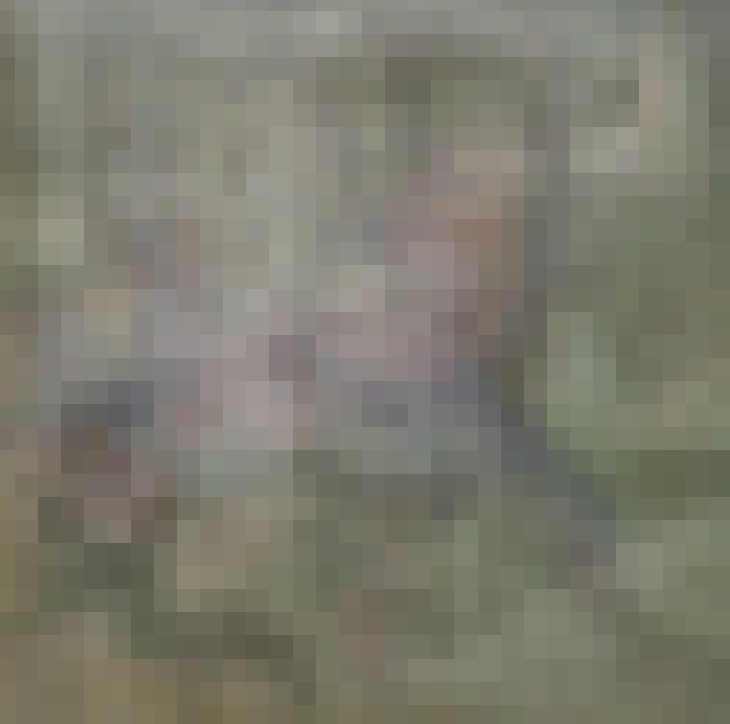
The second and fourth images are generated based on latent variable by the first and third images. The the most right one is generated based on a random noise. We can see that the generated images are nearly the same, which satisfies the symptoms of posterior collapse.

Next, I try to figure out the cause of such phenomenon. I first check latent variables z for first and third images, making sure that they are not 0 and different. However, they are not nearly 0 and are different from each other, meaning that the problem probably lies on the decoder instead of encoder.

I then changed the decoder, adding more linear layers and hoping it can learn more about latent variable. However, it doesn’t work and the generated images are still very blurry and the same for any latent variable z. So, it’s most likely not the fault of decoder.

Later, I examine the loss function which has two parts, reconstruction loss and KL loss. econstruction loss measures whether the generated image matches the original image. KL loss measures whether distribution of latent varaible matches standard Gaussian distribution. During training session, I found out that reconstruction loss is usually 0.2 and remains the same during the process. The KL loss is usually a few hundred initially and then rapidly decreasing to 1 or 2. This stark contrast between reconstruction loss and KL loss is possibly the reason why the model neglects image reconstruction.

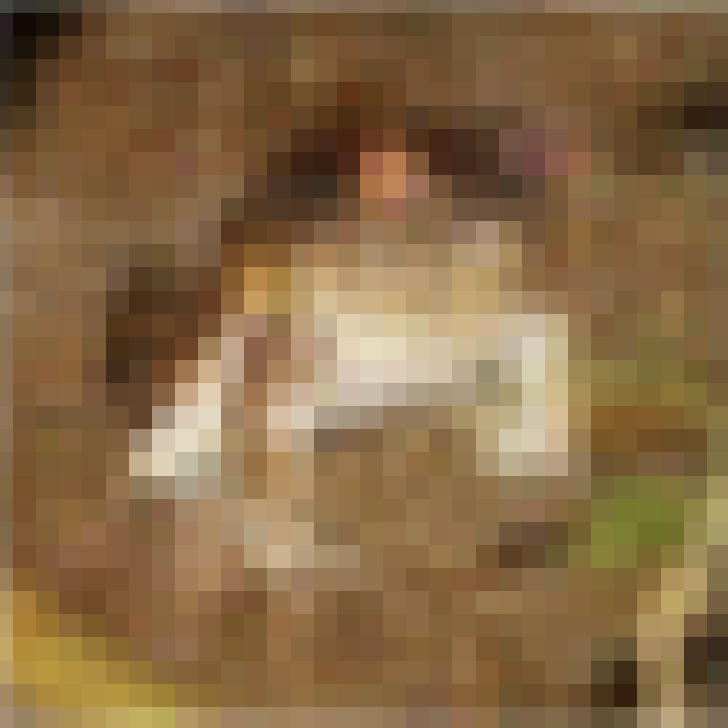
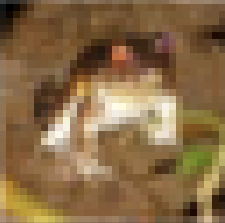
Threfore, I heavily penalized reconstruction loss, multiplying it by 6000. Below are the result after penalizing reconstruction:

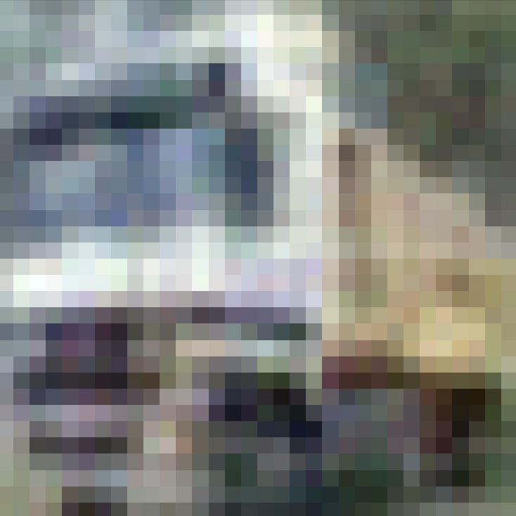
Finally, the model is able to generate discernable image based on the original image, but the generated image is still a bit blurry.